Branch: Specializing Robotics Solvers in Warp

The problem

Maximizing throughput requires kernels specialized to

the robot, the batch, the horizon and even the GPU.

Almost nobody can afford that, so libraries commit to

one elimination plan and one GPU schedule,

and no single choice is best everywhere.

As robot, batch, horizon and GPU vary, the fastest kernel varies (the evidence), and even the best single configuration for a whole map is slower than the per-cell winner by up to 1.5× in single-frame IK, 1.3× in trajectory optimization and 2.7× in contact response (the results).

The solution

An application states its

problem, elimination plan and GPU schedule;

Branch generates the kernel for that configuration.

Because any combination can be generated, specializing to the workload at hand becomes practical.

Branch

The three descriptions are written separately. The application writes the problem: its unknowns, the relations between them, and its residual terms. It chooses an elimination plan and a GPU schedule from the options below. Branch derives the before anything is compiled, then generates the kernel for that configuration.

What fronts, widths, fill, depth and launch count mean

front: a group of unknowns eliminated together with the live unknowns they couple to; each box in the drawings below is a front, and its result enters its parent.
width: how many unknowns a front holds, eliminated plus coupled; it sets the size of the dense block factored at that front and its shared-memory need.
fill: the number of factor entries the plan creates, that is the storage per instance.
depth: the longest chain of fronts that depend on one another, the number of steps that must run one after another.
launch count: how many kernel launches the schedule needs for one solve.

plan   = br.plan(prob, br.order.frames(u, time="cyclic"))   # or br.order.tree(u), br.order.dense(u), time="chronological"
solver = br.compile(plan, br.Schedule.fused(plan))            # or .serial, .levels, .paths, .instance_blocks, .cooperative

Plan which unknowns are eliminated together, and in what order

step 0 of 8

Schedule how the fronts of the tree plan are grouped onto workers and launches; numbers give the processing order waitingrunningdone

Plan: tree dense chronological frames cyclic frames Schedule: Sserial Llevels Ppaths Iinstance blocks Ccooperative Ffused

Colour marks the plan and the letter the schedule, here and in every map below. Launch counts belong to this small illustration and follow the library's grouping rules; fused runs like cooperative on the tree and dense plans, since a block per chain only pays where frames form single-child chains.

The evidence

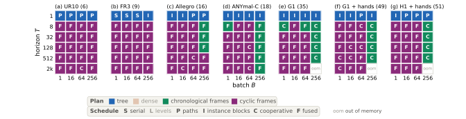
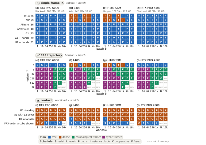
The best plan and schedule vary with robot, batch size, horizon and GPU

Each cell is the fastest Branch configuration for that cell: the colour is the plan and the letter the schedule, as in the legend under each figure. oom marks a cell in which the candidate or its native reference did not fit in device memory. Every figure is rendered by the paper's figure pipeline from the recorded rows.

On a narrow screen each figure scrolls sideways; every figure also opens full size.

Maps of the fastest Branch configuration per cell, one panel per robot, batch by horizon. Cell colour is the plan and the letter the schedule. — **The best plan and schedule move with robot, batch and horizon.** One panel per robot (tangent coordinates in parentheses), batch × horizon on one RTX PRO 6000. The tree plan wins every single-frame IK cell, and only the schedule changes with robot and batch. Over the 137 drawn trajectory cells the cyclic-frames plan wins 114 and the chronological-frames plan 23: cyclic on the two arms everywhere and on the G1 and the H1 at B ≤ 64, chronological on those two at B = 256. The G1's (70;140) and the H1's (51;102) cyclic fronts exceed this GPU's shared memory as one tile factor and are generated as a split factor. The fused schedule wins 113 cells and the cooperative schedule 24; the runner-up is within 3 % in 81. The G1 with hands and the H1 use a velocity-only objective. Open full size.

The single-frame IK map, the FR3 trajectory map and the contact map on four GPUs. Cell colour is the plan and the letter the schedule. — **The best plan and schedule also depend on the GPU.** Row 1 is single-frame IK over robots × batch on four GPUs (architecture, SM count and shared memory per block under each name); panel (a) is the RTX PRO 6000, whose columns are the T = 1 row of the map above. Rows 2 and 3 repeat the FR3 trajectory map and the contact map on each GPU. In single-frame IK the winner changes in 19 of 49 cells on the L40S and 24 of 49 on the H100 (11 and 13 of them beyond the 3 % tie band): the dense plan wins the two arm chains at B ≤ 1024 (8 and 7 cells) and the levels schedule 5 and 7 humanoid cells; on the RTX PRO 4500 one winner changes beyond the tie band. In the FR3 trajectory row the T = 8 winner is mixed on the other GPUs, the cyclic-frames plan at the smallest batches and the chronological-frames plan from B = 64–256 up; over the shared FR3 cells the winner changes beyond the tie band in 2 (L40S), 7 (H100) and 5 (RTX PRO 4500) cells, and within it in 11, 7 and 2. In the contact row the dense plan wins every robot-dominated world on every GPU except the H1 at a table at B = 1 on the L40S and H100 (tree plan, instance blocks), and the FR3 cube shower is the tree plan from B = 64 up wherever it fits in memory (the dense plan at B ≤ 16 on the RTX PRO 6000 and at B = 1 on the RTX PRO 4500); beyond the tie band two (L40S) and three (H100) contact winners change, all at B ≤ 64, and none on the RTX PRO 4500. Open full size.

The three descriptions

Problem, elimination plan, GPU schedule

The problem states the unknowns, the linear relations between them and the residual terms of the local quadratic problem. The elimination plan states which unknowns are eliminated together and in what order. The GPU schedule states how the plan's operations are grouped onto threads, cooperating blocks or tiles, and where storage is placed. br.plan turns a problem and an order into a plan; br.compile turns a plan and a schedule into kernels.

Problem Unknowns, their relations, and residual terms

x_b = X_b x_pa(b) + S_b u_b

residual terms: reach, grasp, smoothness

a trajectory adds frames t, t+1, …

Elimination plan Which unknowns are eliminated together, and in what order

tree

joint by joint along the tree

dense

every joint in one front

chronological frames

frame after frame

cyclic frames

odd frames, then every other

GPU schedule waitingrunningdone Which operations run together, on which workers

serial

one thread per instance

levels

one thread per front

paths

one thread per path

instance blocks

one block per k instances

cooperative

one tile block per front

fused

one tile block per chain

Each box is a front: a group of unknowns eliminated together with the live unknowns they couple to; its result enters its parent. Numbers give each schedule's processing order (solid: running; tinted: done). S–C show the tree plan, F the chronological-frames plan, whose frames form the chains it fuses. The explorer above runs every plan under every schedule.

Interface (Python)

Two excerpts. The first is batched inverse kinematics inside the application's Levenberg–Marquardt loop; the second reuses the same problem over T frames and changes only the plan and the schedule. Kinematics, damping, acceptance and retraction stay in the application.

import warp as wp, warp.branch as br
import newton.ik as ik                                   # kinematics helpers stay in Newton

robot = br.Articulation.from_newton(model)               # topology + body/joint labels
u = br.tangents(robot, instances=B, q=q_dof)             # BlockSet: u_b of width dof[b]
x = br.twists(u, pose=body_q, S=S_cols)                  # BlockSet: x_b = X_b x_parent + S_b u_b

@br.residual
def reach(body: br.Body, target: wp.vec3, point: wp.vec3) -> wp.vec3:
    return target - br.position(body, point)             # Jacobian by in-kernel autodiff

@br.residual
def limit(d: br.Dof, lo: float, hi: float) -> float:
    v = d.q + d.value
    return wp.max(v - hi, 0.0) + wp.max(lo - v, 0.0)

prob = br.Problem()
prob.add(reach, body=x[hand_names], target=pos_targets, point=wp.vec3(), weight=t_weights)
prob.add(limit, d=u.dofs, lo=model.joint_limit_lower, hi=model.joint_limit_upper, weight=10.0)
prob.add(br.damping(u, weight=lam))                      # H += lam I on every tangent block

plan   = br.plan(prob, br.order.tree(u))                 # the tree plan: fronts [u_b ; x_parent(b)]
sched  = br.Schedule.instance_blocks(plan)               # one cooperative block per k instances
solver = br.compile(plan, sched, device=dev)
print(plan.report()); print(sched.report())              # widths, fill, depth, launches: before any kernel runs

for it in range(24):                                     # the application owns the nonlinear loop
    ik.fill_kinematics(model, joint_q, body_q, S_cols, q_dof)
    solver.linearize(); solver.factor()
    solver.solve().dofs(u, out=dq)                       # z = -H^-1 g, compact [B, n]
    ik.retract_dofs(model, joint_q, dq, joint_q)

T = 128
u = br.tangents(robot, instances=B, frames=T, q=q_dof)   # BlockSet (bodies, T); arrays [B, T, ...]
x = br.twists(u, pose=body_q, S=S_cols)

@br.residual
def smooth(a: br.Dof, b: br.Dof, inv_dt: float) -> float:
    return ((b.q + b.value) - (a.q + a.value)) * inv_dt

prob = br.Problem()
prob.add(reach,  body=x[hand_names, :], target=hand_targets, point=wp.vec3(), weight=8.0)
prob.add(smooth, a=u.dofs[:, :-1], b=u.dofs[:, 1:], inv_dt=30.0, weight=0.05)     # temporal edges by slicing
prob.add(br.damping(u, weight=lam))

# Same problem, other plans. Nothing else changes.
plan_chron = br.plan(prob, br.order.frames(u, time="chronological"))  # chronological frames: fronts [U_t ; U_t+1]
plan_cyc   = br.plan(prob, br.order.frames(u, time="cyclic"))         # cyclic frames: odd frames first
print(plan_cyc.report())                                              # classes, widths, levels, storage

# Same plan, several schedules. Same factorization, different mapping.
for sched in (br.Schedule.levels(plan_cyc),                           # thread per (instance, front)
              br.Schedule.cooperative(plan_cyc, block_dim=64),        # tile block per (instance, front)
              br.Schedule.fused(plan_cyc, block_dim=64)):             # block per (instance, chain), tiles resident
    solver = br.compile(plan_cyc, sched, device=dev)
    print(sched.report())                                             # launches per phase, kernels, shared memory

The trajectory integration in the paper receives Newton's assembled frame blocks as by-reference quadratic terms instead of the residuals shown here; the plan and schedule calls are the same.

Named libraries and algorithms

Existing solvers commit to one elimination plan and one GPU schedule

Existing solvers commit to one of these choices when they are written; the table lists the plan and the schedule each one fixes, and a dash or CPU where the choice does not exist or is not stated. Branch generates any of the four plans under any of the six schedules of the legend from one problem description.

Library or algorithm	Elimination plan	GPU schedule	What is fixed
Algorithms
Articulated-body algorithm	tree	—	leaf-to-root Schur-complement recursion over the kinematic tree
Composite-rigid-body algorithm with dense Cholesky	dense	—	forms the dense joint-space inertia, then factors it
Riccati recursion / block-Thomas (DDP backward pass)	chronological frames	—	eliminates frames in time order
Cyclic reduction	cyclic frames	—	eliminates every other frame, ceil(log2 T)+1 levels
Libraries and solvers
LoIK	tree	CPU	articulated-body recursion applied to differential IK, CPU implementation
GRiD	tree	Llevels	URDF-specialized CUDA, one wave per tree level
cuRobo	dense	Ccooperative	traversal, threads per problem and shared-memory layout fixed at compile time; dense normal matrix
MuJoCo Warp	dense	own kernels	joint-space mass matrix; scalar, tiled or sparse factorization picked per model from preprocessed block structure
PhysX articulations	tree	own kernels	reduced-coordinate articulations; impulse response with per-articulation kernels
Newton single-frame IK (IKOptimizerLM)	dense	Ccooperative	damped normal equations J^T J + lambda I with a tiled dense Cholesky in one fused LM kernel
Newton physics engine projected-Gauss–Seidel contact solver, joint-space response	dense	own kernels	joint-space response columns Y = M^-1 J^T once per step, per-articulation kernels
Newton physics engine projected-Gauss–Seidel contact solver, per-body response (propagation)	tree	own kernels	per-body 6x6 response blocks, impulses propagated along the tree each sweep, per-articulation kernels
Newton trajectory IK, direct solver	chronological frames	Ccooperative	block-tridiagonal Cholesky over superblocks held in shared memory
SOCU	cyclic frames	—	GPU block-tridiagonal Cholesky by nested dissection; thread mapping not stated in its paper
MPCGPU	other / iterative	—	preconditioned conjugate gradient on the Schur system
PyRoki / jaxls	other / iterative	own kernels	user residuals over a JAX least-squares solver; joint-space dense Cholesky or conjugate gradient per call (the CG path is the drawn humanoid trajectory row), XLA kernels
pytorch_kinematics	dense	own kernels	damped-least-squares single-frame IK as a Python loop of small kernels
GMR	other / iterative	CPU	motion retargeting on the CPU one frame at a time
GTSAM	other / iterative	CPU	elimination tree from any variable ordering; CPU
Ceres	other / iterative	own kernels	Schur elimination or sparse Cholesky, interchangeable per solve; CPU, with CUDA dense and cuDSS solvers in the cited 2.2 release
Branch	tree, dense, chronological frames, cyclic frames	S L P I C F	one planner and one kernel generator; any of the four plans under any of the six schedules, chosen by name

Plans and schedules as named in the paper's related work. A dash marks a GPU schedule that does not exist (an algorithm, or a CPU library) or one that its paper does not state. Branch plans on the lifted articulated space, so the tree recursion, joint-space condensation and the temporal orderings are one representation with one executor.

Applications

Demonstrated on inverse kinematics, from single poses to trajectories, and on contact response

Branch is a library for the structured linear solves at the core of robotics optimizers and simulators; this paper demonstrates it on inverse kinematics, from single poses to trajectories, and on contact response inside a Newton physics engine projected-Gauss–Seidel contact solver. With generated kernels in place of the hand-written ones, the contact solver runs at or above its native throughput: end to end, the dense-plan adapter runs the Isaac Lab G1 velocity task at 1.02× and 1.03× the native environment-step throughput at B = 4096 / 16384; at matched accuracy single-frame IK is 4.6–128× faster than PyRoki and 5–21× faster than pytorch_kinematics; trajectory optimization at B = 1 is faster than PyRoki/jaxls on every robot at every measured horizon: 5.8–111× on the UR10, FR3, Allegro and ANYmal-C, and 2.2–4.2× on the G1 and 2.7–4.0× on the H1 once their wide fronts are generated as a split factor. Each integration fixes what stays in the application and what Branch generates, and each exposes a different decision.

Single-frame IK Inverse kinematics

What is solved: Newton's batched Levenberg–Marquardt optimizer forms the damped normal equations (J^ᵀJ + λI) δ = −J^ᵀr of its position, rotation and joint-limit residuals and accepts or rejects each step.
Branch generates: Residual evaluation, the Jacobian step and the linear solve. The outer loop, damping, step acceptance and retraction are inherited from Newton.
The decision: The plan (tree or dense) and, within it, any of the six schedules. The robot changes the front tree, the batch changes the parallel work per launch.
Measured: At matched accuracy Branch is 4.6–128× faster than PyRoki (4.6–7.6× at B = 1, 38–108× at B = 16384; the largest ratio is the H1 + hands at B = 4096) and 5–21× faster than pytorch_kinematics.
Per-robot ratios
On the UR10, Branch is 6.9–60× faster than PyRoki at B ∈ {1, 16, 64, 256, 1024, 4096, 16384}. On the FR3, Branch is 5.1–38× faster than PyRoki at B ∈ {1, 16, 64, 256, 1024, 4096, 16384}. On the Allegro, Branch is 7.6–103× faster than PyRoki at B ∈ {1, 16, 64, 256, 1024, 4096, 16384}. On the ANYmal-C, Branch is 4.6–48× faster than PyRoki at B ∈ {1, 16, 64, 256, 1024, 4096, 16384}. On the G1, Branch is 4.8–79× faster than PyRoki at B ∈ {1, 16, 64, 256, 1024, 4096, 16384}. On the G1 + hands, Branch is 5.1–107× faster than PyRoki at B ∈ {1, 16, 64, 256, 1024, 4096, 16384}. On the H1 + hands, Branch is 5.2–128× faster than PyRoki at B ∈ {1, 16, 64, 256, 1024, 4096, 16384}. Against pytorch_kinematics (damped least squares, 24 iterations), Branch is 12–21× faster on the UR10 at B ∈ {1, 256, 4096, 16384} and 5.1–16× faster on the FR3 at B ∈ {1, 256, 4096, 16384}.

Trajectory Trajectory optimization

What is solved: Trajectory IK chooses joint configurations q₀, …, q_T−1 that track pose targets under smoothness, limit and posture penalties: the same LM iteration over T frames, and a single pose is the case T = 1.
Branch generates: The factorization and substitution of the assembled block-tridiagonal system, received as by-reference quadratic terms on the free frame blocks. Newton assembles the per-frame blocks and masks fixed and padded frames.
The decision: The temporal order (chronological or cyclic frames) and the schedule (Ccooperative or Ffused). The horizon sets depth and width; the GPU's shared memory decides whether a cyclic front is factored as one tile or as a split factor.
Measured: At B = 1 Branch is 5.8–111× faster than PyRoki/jaxls on the UR10, FR3, Allegro and ANYmal-C at every measured horizon, 3.3–18× on the G1 + hands at T ≤ 128, and 2.2–4.2× on the G1 and 2.7–4.0× on the H1 + hands at every measured horizon; on the G1 and H1 + hands the cyclic-frames plan's fronts exceed this GPU's shared memory as one tile factor, so the kernel generator emits them as a split factor (an in-place Cholesky and lower solve, then a row-blocked Schur update) and the plan fits.
Per-robot ratios
On the UR10, PyRoki/jaxls on the matched objective is 7.0–9.5× slower than the best Branch configuration up to T = 128 and 32–35× slower than the best Branch configuration from T = 512 on. On the FR3, PyRoki/jaxls on the matched objective is 6.7–9.0× slower than the best Branch configuration up to T = 128 and 99–111× slower than the best Branch configuration from T = 512 on. On the Allegro, PyRoki/jaxls on the matched objective is 6.8–11× slower than the best Branch configuration up to T = 128 and 15–21× slower than the best Branch configuration from T = 512 on. On the ANYmal-C, PyRoki/jaxls on the matched objective is 5.8–9.2× slower than the best Branch configuration up to T = 128 and 22–27× slower than the best Branch configuration from T = 512 on. On the G1, PyRoki/jaxls on the matched objective is 2.8–4.2× slower than the best Branch configuration up to T = 128 and 2.2–2.8× slower than the best Branch configuration from T = 512 on. On the G1 + hands, PyRoki/jaxls on the matched objective is 3.3–18× slower than the best Branch configuration up to T = 128. On the H1 + hands, PyRoki/jaxls on the matched objective is 3.5–4.0× slower than the best Branch configuration up to T = 128 and 2.7–3.0× slower than the best Branch configuration from T = 512 on.

Contact Contact response

What is solved: Inside a Newton physics engine projected-Gauss–Seidel contact solver, every sweep needs how an impulse on one body changes the joint velocities of the whole robot. The solver's two response strategies are two plans of one problem: the dense plan forms the joint-space response columns once per step; the tree plan keeps per-body 6 × 6 response blocks and propagates impulses along the tree once per sweep.
Branch generates: The factorization and the response operations of either plan, from one problem statement of the robot's inertia. Collision detection, row construction, friction, the sweeps and integration stay in the solver.
The decision: The plan (dense or tree) and, within it, the schedule. The workload and the number of worlds decide: the dense plan wins every robot-dominated world, and the cube piles switch from the dense plan at small batch to the tree plan from B = 64 (cube shower) or B = 1024 (falling cubes) up.
Measured: With generated kernels in place of the hand-written ones, the contact solver runs at or above its native throughput. End to end, the dense-plan adapter runs the Isaac Lab G1 velocity task at 1.02× and 1.03× the native environment-step throughput at B = 4096 / 16384, and the physics step at 1.00× and 1.02×.

Complete results

What the measurements show

Four questions, answered separately: which Branch configuration is fastest for a given robot, batch, horizon or contact workload, and how the answer moves with the GPU; how much choosing correctly matters; how the fastest configuration compares with external baselines and with the hand-written kernels; and what trying an alternative costs. Every figure and number below is rendered by the paper's figure pipeline from the recorded rows.

Protocol. One NVIDIA RTX PRO 6000 Blackwell GPU unless stated, forks of Warp and Newton, float32 device arithmetic, float64 host oracles. Each timed region is captured into a CUDA graph and replayed warm; medians are reported, excluding compilation and transfers. Timed boundaries are complete application work: a 24-iteration LM solve for single-frame IK, a 32-iteration LM solve including native assembly for trajectory optimization, and one collision-plus-solver substep on B worlds for contact. A row enters a figure only if it passes a matched-accuracy gate (within 1 mm) against the native implementation of its cell. The single-frame IK maps cover 7 robots (UR10 (6), FR3 (9), Allegro (16), ANYmal-C (18), G1 (35), G1 + hands (49) and H1 + hands (51); tangent coordinates in parentheses) at B ∈ {1, 16, 64, 256, 1024, 4096, 16384}; the trajectory maps cover B ∈ {1, 16, 64, 256} × T ∈ {8, 32, 128, 512, 2048} on 7 robots, and B ∈ {1024, 4096, 16384} on the FR3; the contact maps cover 10 workloads at 1 to 262,144 worlds.

On a narrow screen each figure scrolls horizontally; every figure also opens full size.

Q1 Which configuration wins?

The maps above show the fastest Branch configuration that passed the gate in every cell: colour is the plan and the letter the schedule. oom marks a cell in which the candidate or its native reference did not fit in device memory. Native rows never enter a map.

Motion cells won per configuration

(a) UR10, batch × horizon (T = 1 included): 24 of 24 measured cells have a winner; wins by plan: tree 4, cyclic frames 20; by configuration: cyclic / fused 19, tree / paths 4, cyclic / cooperative 1; the runner-up is within 3 % in 13.
(b) FR3, batch × horizon (T = 1 included, all 7 batches; the figure draws B ≤ 256): 39 of 39 measured cells have a winner; wins by plan: tree 7, cyclic frames 20, chronological frames 12; by configuration: cyclic / fused 20, chronological / fused 6, chronological / cooperative 6, tree / serial 4, tree / instance_blocks 3; the runner-up is within 3 % in 23; 3 oom cells (the candidate or its native reference did not fit in memory).
(c) Allegro, batch × horizon (T = 1 included): 24 of 24 measured cells have a winner; wins by plan: tree 4, cyclic frames 17, chronological frames 3; by configuration: cyclic / fused 15, chronological / fused 3, tree / instance_blocks 2, cyclic / cooperative 2, tree / paths 2; the runner-up is within 3 % in 17.
(d) ANYmal-C, batch × horizon (T = 1 included): 24 of 24 measured cells have a winner; wins by plan: tree 4, chronological frames 6, cyclic frames 14; by configuration: cyclic / fused 12, chronological / fused 6, tree / instance_blocks 4, cyclic / cooperative 2; the runner-up is within 3 % in 17.
(e) G1, batch × horizon (T = 1 included): 23 of 23 measured cells have a winner; wins by plan: tree 4, chronological frames 6, cyclic frames 13; by configuration: cyclic / fused 13, chronological / cooperative 5, tree / instance_blocks 4, chronological / fused 1; the runner-up is within 3 % in 7; 1 oom cell (the candidate or its native reference did not fit in memory).
(f) G1 + hands (velocity-only objective), batch × horizon (T = 1 included): 23 of 23 measured cells have a winner; wins by plan: tree 4, cyclic frames 15, chronological frames 4; by configuration: cyclic / fused 9, cyclic / cooperative 6, chronological / cooperative 4, tree / instance_blocks 3, tree / paths 1; the runner-up is within 3 % in 18; 1 oom cell (the candidate or its native reference did not fit in memory).
(g) H1 + hands (velocity-only objective), batch × horizon (T = 1 included): 23 of 23 measured cells have a winner; wins by plan: tree 4, cyclic frames 15, chronological frames 4; by configuration: cyclic / fused 15, chronological / cooperative 4, tree / paths 3, tree / instance_blocks 1; the runner-up is within 3 % in 3; 1 oom cell (the candidate or its native reference did not fit in memory).

In contact response the plan changes with the workload and, on the cube piles, with the number of worlds. The contact map is the third row of the GPU figure above (workload × worlds, one collision-plus-solver substep). The dense plan wins all 29 robot-dominated cells (a standing G1 to 262,144 worlds, G1 with twelve boxes, H1 at a table) and the four Isaac Lab tasks at 4096 environments. Of the 21 FR3 cube-pile cells, 11 go to the tree plan and 10 to the dense plan (one of those in the tree elimination order): the dense plan at small batch, the tree plan from B = 64 (cube shower) or B = 1024 (falling cubes) up. In most cells the runner-up is another schedule or block size of the same plan; the plan is the decision that matters: the best single configuration for the map, dense / cooperative, is up to 2.7× slower than the per-cell winner (cube shower, B = 4096, where tree / serial wins), while the schedule is worth at most 3 % except at small batches of the tree plan.

Contact cells won per configuration

Contact response, workload × worlds: 54 of 54 measured cells have a winner; wins by plan: dense 42, tree 11, dense (tree order) 1; by configuration: dense / cooperative 42, tree / instance_blocks 8, tree / serial 2, dense (tree order) / instance_blocks (rhs tile 4) 1, tree / levels (rhs tile 4) 1; the runner-up is within 3 % in 45; 3 oom cells (the candidate or its native reference did not fit in memory).

Q2 How much does choosing correctly matter?

Two prices of a wrong choice, as time ratios over the cells of each map. Second best is the runner-up over the winner. One fixed configuration is the best single configuration for the whole map, the one that passes in at least 90 % of the cells with the best geometric-mean ratio, over the per-cell winner; this is the only ratio on this page that measures the cost of not specializing.

Application	Cells	Runner-up within (median · worst)	One fixed configuration	costs up to	where
single-frame IK	49	4 % · 14 %	`tree / instance_blocks` (no passing row in 1 cell)	1.53×	H1 + hands, B = 4096, where `tree / paths` wins
trajectory (FR3)	32	2 % · 17 %	`cyclic / fused`	1.34×	B = 16384, T = 128, where `chronological / cooperative` wins
contact	54	0.2 % · 2.03×	`dense / cooperative`	2.67×	cube shower, 1 s, B = 4096, where `tree / serial` wins
trajectory (all robots, T ≥ 8)	149	3 % · 4.70×	`cyclic / fused`	1.34×	FR3, B = 16384, T = 128, where `chronological / cooperative` wins

A near miss costs a few percent on median; even the best single configuration is up to 1.5× slower than the per-cell winner in single-frame IK, 1.3× across the trajectory maps and 2.7× across the contact map. The second-best candidate is within 4 % (single-frame IK), 2 % (trajectory (FR3)), 0.2 % (contact) and 3 % (trajectory (all robots, T ≥ 8)) of the winner on median. Even the best single configuration for a whole map (the one that passes in at least 90 % of the cells with the best geometric-mean ratio) is slower than the per-cell winner by up to 1.5× (single-frame IK), 1.3× (trajectory (FR3)), 2.7× (contact) and 1.3× (trajectory (all robots, T ≥ 8)), and where it has no passing row it fails outright. On the FR3 trajectories drawn above (B ≤ 256) the cyclic-frames plan wins every cell; at B ≥ 1024 the chronological-frames plan takes over (12 of the 32 FR3 cells). Fixing the best single configuration, cyclic / fused, for every robot costs at most 1.3× against the per-cell winner, at B = 16384, T = 128 on the FR3; on the humanoids the two orders are far apart, and the runner-up at B = 16, T = 2048 on the H1 is the chronological order at 4.7× the cyclic-frames time.

GPU Does the map move with the GPU?

The GPU figure above repeats the single-frame IK map, the FR3 trajectory map and the contact map on an H100, an L40S and an RTX PRO 4500 next to the RTX PRO 6000 of the other figures. The single-frame IK winner changes in 19 of 49 cells on the L40S and 24 of 49 on the H100, 11 and 13 of them beyond the 3 % tie band; the dense plan appears on the two arm chains at B ≤ 1024 and the levels schedule on the humanoids (5 and 7 cells). On the RTX PRO 4500 one single-frame IK winner changes beyond the tie band. In contact response two winners change beyond the tie band on the L40S and three on the H100, all at B ≤ 64, and none on the RTX PRO 4500. The H100's 227 KiB of shared memory per block hold the G1 cyclic-frames trajectory plan as one tile factor, where the RTX PRO 6000's 99 KiB take the split factor; there too it wins every T ≥ 32 cell, by 1.3–4.0× over the chronological order.

Q3 How competitive is the fastest configuration?

External libraries are kept out of the maps and compared in their own plot at matched accuracy; every Branch point is its fastest gate-passing configuration in that cell. In single-frame IK every solver starts from the same 17 configurations per problem (the nominal pose and 16 sampled within the joint limits), runs 24 iterations from each and keeps the best solution by the matched cost; the time is the whole multi-start solve per problem.

Milliseconds per solve on a log axis, two rows of panels, one per robot: single-frame IK against batch, then trajectory optimization against horizon. Branch's fastest configuration against PyRoki and pytorch_kinematics. — In single-frame IK Branch is 4.6–128× faster than PyRoki and 5–21× faster than pytorch_kinematics at matched accuracy; in trajectory optimization it is faster than PyRoki/jaxls on every robot at every horizon: 5.8–111× on the UR10, FR3, Allegro and ANYmal-C, 2.2–4.2× on the G1 and 2.7–4.0× on the H1. Milliseconds per complete solve on a log axis, lower is faster; every measured point is drawn. Row A: single-frame IK against batch, one panel per robot; each point is the whole multi-start solve of the batch. Row B: trajectory optimization at B = 1 against horizon (32 iterations, native assembly included); PyRoki/jaxls solves the matched objective on every robot. Series: Branch, PyRoki (matched residuals) and pytorch_kinematics (damped least squares). With 17 starts every Branch and native row passes the accuracy gate (within 1 mm); PyRoki misses once (UR10, B = 256, 3 mm) and pytorch_kinematics misses on the FR3 from B = 256 (3–12 mm). The G1 with hands and the H1 use the velocity-only objective. On the G1 and H1 the cyclic-frames plan's (70;140) and (51;102) fronts exceed this GPU's shared memory as one tile factor, so the kernel generator emits them as a split factor, an in-place Cholesky and lower solve followed by a row-blocked Schur update, whose widest step needs 78,400 B and 62,432 B; the plan then fits and is the drawn Branch row at every T except the G1's T = 8. Open full size.

Against external libraries

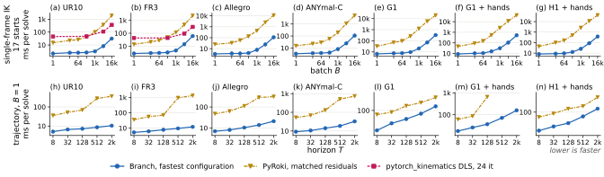
In single-frame IK Branch is 4.6–128× faster than PyRoki (4.6–7.6× at B = 1, 38–108× at B = 16384; the largest ratio is the H1 + hands at B = 4096) and 5–21× faster than pytorch_kinematics on the UR10 and the FR3. In trajectory optimization at B = 1 Branch is faster than PyRoki/jaxls on every robot at every measured horizon: 5.8–111× on the UR10, FR3, Allegro and ANYmal-C, 3.3–18× on the G1 with hands at T ≤ 128, and 2.2–4.2× on the G1 and 2.7–4.0× on the H1, whose (70;140) and (51;102) cyclic fronts exceed this GPU's shared memory as one tile factor and are generated as a split factor: an in-place Cholesky and lower solve, then a row-blocked Schur update, so the kernel needs only its widest step (78,400 B on the G1, 62,432 B on the H1). The per-cell ratios are listed with the applications; the figure carries every library with recorded rows.

Against the hand-written kernels

Inside the contact solver, the generated kernels leave throughput at or above native: end to end, the dense-plan adapter runs the Isaac Lab G1 velocity task at 1.02× and 1.03× the native environment-step throughput at B = 4096 / 16384 and the physics step at 1.00× and 1.02×. The single-frame IK and trajectory rows are compared with external libraries only.

Q4 What does trying an alternative cost?

What a new configuration costs before its first timed step, as ranges over the configurations of each application. Plan: symbolic planning and the reports. Compile: kernel generation, JIT and module load, from scratch (cold cache) and with the kernels already in Warp's kernel cache (warm; the single-frame IK sweep records a cache hit as 0.0 at 0.1 s resolution); for the contact adapters it is the constructor total, which they record as a whole. First call: module load and first launch. Kernels: generated kernels per configuration.

Application	Configurations	Plan (ms)	Compile, cold (s)	Compile, warm (s)	First call (ms)	Kernels
single-frame IK (G1)	16	1.7–2.2	3.2–209.7	0.0	10–30	3–9
trajectory (FR3, T = 128)	8	8.5–10.6	5.7–32.7	0.02–0.54	38–954	3–21
contact (G1)	8	—	2.8–241.3	0.02	—	—

Per-configuration rows

Application	Configuration	Plan (ms)	Compile, cold (s)	Compile, warm (s)	First call (ms)	Kernels
single-frame IK	`tree / serial`	2.0	204.6	—	10	3
single-frame IK	`tree / levels`	1.8	32.5	—	20	9
single-frame IK	`tree / paths`	1.8	66.4	—	10	9
single-frame IK	`tree / instance_blocks`	1.7	209.7	—	10	3
single-frame IK	`tree / cooperative`	2.0	3.2	—	30	9
single-frame IK	`tree / cooperative (spec)`	1.9	37.0	—	20	9
single-frame IK	`tree / fused`	1.7	—	0.0	30	9
single-frame IK	`tree / fused (spec)`	1.8	—	0.0	20	9
single-frame IK	`dense / serial`	1.9	64.1	—	30	3
single-frame IK	`dense / levels`	2.1	—	0.0	20	3
single-frame IK	`dense / paths`	2.0	—	0.0	20	3
single-frame IK	`dense / instance_blocks`	2.0	59.9	—	20	3
single-frame IK	`dense / cooperative`	2.1	4.6	—	10	3
single-frame IK	`dense / cooperative (spec)`	2.2	12.5	—	10	3
single-frame IK	`dense / fused`	2.0	—	0.0	10	3
single-frame IK	`dense / fused (spec)`	2.0	—	0.0	10	3
trajectory	`chronological / fused (block 64)`	8.5	15.4	0.16	43	3
trajectory	`chronological / fused (block 128)`	8.9	17.4	0.19	38	3
trajectory	`cyclic / fused (block 64)`	9.8	32.7	0.54	50	9
trajectory	`cyclic / fused (block 128)`	10.6	32.5	0.45	49	9
trajectory	`chronological / cooperative (block 64)`	9.4	13.5	0.23	153	6
trajectory	`cyclic / cooperative (block 64)`	9.8	21.9	0.38	52	9
trajectory	`chronological / levels`	8.5	5.7	0.02	954	6
trajectory	`cyclic / levels`	10.2	11.0	0.03	371	21
contact	`dense plan (dense order) cooperative:128`	—	2.8	0.02	—	—
contact	`dense plan (dense order) cooperative:256`	—	10.6	0.02	—	—
contact	`dense plan (tree order) instance_blocks` (rhs tile 4)	—	154.9	0.02	—	—
contact	`dense plan (tree order) levels` (rhs tile 4)	—	3.9	0.02	—	—
contact	`tree plan instance_blocks`	—	229.2	0.02	—	—
contact	`tree plan levels` (rhs tile 4)	—	38.3	0.02	—	—
contact	`tree plan paths`	—	77.2	0.02	—	—
contact	`tree plan serial`	—	241.3	0.02	—	—

Planning costs milliseconds, compiling seconds to minutes. The reports exist after planning, so an infeasible plan is refused before compilation. Compilation is the real cost: table-driven register kernels and tile kernels compile in seconds, plan-specialized register kernels in minutes because every front is unrolled with literal offsets. A compiled configuration serves every batch. This is the cost that replaces a new derivation and a new hand-written kernel.

Scope

Scope and limits

Branch's plans are known Schur-complement recursions and its schedules known GPU mappings; what is new is that one problem description, one planner and one kernel generator produce the kernel for any plan and schedule named on this page, so a developer can ask before compiling how wide the fronts are, how deep the chain is and what a mapping costs, and can change the answer with one line.

Branch does not choose the configuration. The maps are measured, and the plan report describes fill, depth and storage rather than predicting runtime. Crossover points move with the GPU.
Trying an alternative is not free. Each configuration is planned and then compiled as a specialized kernel (Q4). This is the cost that replaces a new derivation and a new hand-written kernel.
The application owns the outer loop. Branch solves the local quadratic; Gauss–Newton or LM iteration, damping, acceptance, retraction, contact sweeps and kinematics stay in the application, and warp.branch never imports Newton.
Gradients stop at the local quadratic. Residuals are differentiated to build the system; nothing differentiates through factor or solve.
Orders are recipes. Orders are recipes (tree, dense, frames, eliminate, concatenation) plus explicit elimination; there is no minimum-degree or nested-dissection heuristic. A plan whose storage exceeds the memory budget is refused with its report attached.
Kinematic trees, float32. Loop-closing joints inside an articulation are unsupported. Device arithmetic is single precision and a failed pivot is flagged rather than repaired; a float64 host oracle backs every plan × schedule in the tests.

Reproducibility

The maps and the results section are generated from the recorded rows. paper/figures/build_all.py reads the recorded rows of the single-frame IK, trajectory, contact and external-baseline sweeps, draws the maps and baseline plots, computes the two tables and lists every consumed file in its manifest; experiments/branch/site_assets.py re-runs that pipeline, renders the figures for this page and fills every generated block from the same manifest. This page was rendered from 346 recorded row files (17 single-frame IK row files; 9 trajectory row files; 1 trajectory-rows-grid-fill file; 2 trajectory-rows-gate-repair files; 2 trajectory-rows-humanoid-b1 files; 1 trajectory-rows-oom file; 1 contact-map file; 44 contact-rows (summarised in map.json) files; 1 contact-grid-fill file; 12 contact-grid-fill (summarised in its map.json) files; 1 contact-oom file; 17 gpu-l40s-ik files; 1 gpu-l40s-ik-gate-repair file; 1 gpu-l40s-trajectory file; 1 gpu-l40s-trajectory-grid-fill file; 1 gpu-l40s-trajectory-final-revision file; 1 gpu-l40s-contact-map file; 15 gpu-l40s-contact-rows (summarised in map.json) files; 1 gpu-l40s-contact-grid-fill file; 7 gpu-l40s-contact-grid-fill (summarised in its map.json) files; 1 gpu-l40s-contact-oom file; 19 gpu-h100-ik files; 1 gpu-h100-ik-gate-repair file; 2 gpu-h100-trajectory files; 1 gpu-h100-trajectory-grid-fill file; 1 gpu-h100-trajectory-final-revision file; 1 gpu-h100-contact-map file; 17 gpu-h100-contact-rows (summarised in map.json) files; 1 gpu-h100-contact-grid-fill file; 7 gpu-h100-contact-grid-fill (summarised in its map.json) files; 1 gpu-h100-contact-oom file; 17 gpu-rtx4500-ik files; 1 gpu-rtx4500-trajectory file; 1 gpu-rtx4500-trajectory-grid-fill file; 1 gpu-rtx4500-trajectory-final-revision file; 1 gpu-rtx4500-contact-map file; 18 gpu-rtx4500-contact-rows (summarised in map.json) files; 1 gpu-rtx4500-contact-grid-fill file; 7 gpu-rtx4500-contact-grid-fill (summarised in its map.json) files; 1 gpu-rtx4500-contact-oom file; 29 external single-frame IK row files; 2 external-ik-gate-repair files; 3 external-socu-ik files; 24 external-trajectory files; 1 ik-multistart file; 49 external-ik-multistart files; 1 plan and compile times file; 1 compile-records file). Every one of them is a final row. The explorer is an illustration whose launch counts follow the same grouping rules as the library.

Branch

The problem

The solution

Branch

The best plan and schedule vary with robot, batch size, horizon and GPU

Problem, elimination plan, GPU schedule

1 Problem Unknowns, their relations, and residual terms

2 Elimination plan Which unknowns are eliminated together, and in what order

3 GPU schedule waitingrunningdone Which operations run together, on which workers

Existing solvers commit to one elimination plan and one GPU schedule

Demonstrated on inverse kinematics, from single poses to trajectories, and on contact response

Single-frame IK Inverse kinematics

Trajectory Trajectory optimization

Contact Contact response

What the measurements show

Q1 Which configuration wins?

Q2 How much does choosing correctly matter?

GPU Does the map move with the GPU?

Q3 How competitive is the fastest configuration?

Against external libraries

Against the hand-written kernels

Q4 What does trying an alternative cost?

Scope and limits

Problem Unknowns, their relations, and residual terms

Elimination plan Which unknowns are eliminated together, and in what order

GPU schedule waitingrunningdone Which operations run together, on which workers